Page 271 - 360.revista de Alta Velocidad - Nº 5

Calculation and rational dimensioning of railway infrastructure materials using numerical modelling

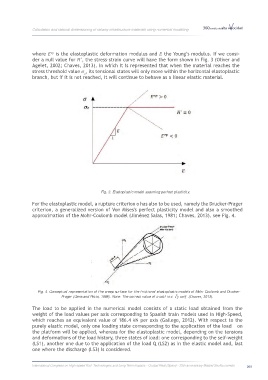
where is the elastoplastic deformation modulus and the Young’s modulus. If we consi-

der a null value for ´, the stress-strain curve will have the form shown in Fig. 3 (Oliver and
Agelet, 2002; Chaves, 2013), in which it is represented that when the material reaches the
stress threshold value , its tensional states will only move within the horizontal elastoplastic

branch, but if it is not reached, it will continue to behave as a linear elastic material.

Fig. 3. Elastoplastic model assuming perfect plasticity.

For the elastoplastic model, a rupture criterion o has also to be used, namely the Drucker-Prager
criterion, a generalized version of Von Mises's perfect plasticity model and also a smoothed
approximation of the Mohr-Coulomb model (Jiménez Salas, 1981; Chaves, 2013), see Fig. 4.

Fig. 4. Conceptual representation of the creep surface for the frictional elastoplastic models of Mohr Coulomb and Drucker-
Prager (Gens and Potts, 1988). Note: The correct value of c·cotf is c √ 3 cotf (Chaves, 2013).

The load to be applied in the numerical model consists of a static load obtained from the
weight of the load values per axis corresponding to Spanish train models used in High-Speed,
which reaches an equivalent value of 186.4 kN per axis (Gallego, 2012). With respect to the
purely elastic model, only one loading state corresponding to the application of the load on
the platform will be applied, whereas for the elastoplastic model, depending on the tensions
and deformations of the load history, three states of load: one corresponding to the self-weight
(LS1), another one due to the application of the load Q (LS2) as in the elastic model and, last
one where the discharge (LS3) is considered.

International Congress on High-speed Rail: Technologies and Long Term Impacts - Ciudad Real (Spain) - 25th anniversary Madrid-Sevilla corridor 269